Chaos: The Double Pendulum

This project looks at the concept of chaos, giving a general introduction to the theory behind it before applying it to a (relatively) simple chaotic system: the double pendulum. We will only consider a frictionless, undriven, and undamped double pendulum where the pendulum lengths are assumed to be rigid and massless. Using a computer simulation of the motion of a double pendulum which traces out the path of the second pendulum, it is clear that the motion of this system is chaotic and highly dependent on initial conditions, illustrating the hallmark characteristics of chaotic systems.

Introduction

Chaos theory is an interdisciplinary branch of mathematics that studies the “chaotic” and complex behavior of dynamical, deterministic systems. To establish some terminology, a deterministic system is defined as one where no randomness is involved in the production of its future states, so given the same initial conditions, our equations of motion will always give us the same output. For the physical laws and systems that we have been studying so far, it is easy to see that the differential equations used to express our equations of motion represent a deterministic system. Theoretically, if we knew the precise initial conditions for a desired system, we could precisely predict the system’s state at some arbitrary point in the future; however, even though a system is deterministic, it does not necessarily mean that its behavior is predictable. Such systems are known as chaotic systems and are characterized by extreme sensitivity to initial conditions where a slight deviation in the initial state of the system results in large differences in a future state. This is also known as the “butterfly effect,” an analogy where a flap of a butterfly’s wings causes a tiny perturbation in initial conditions, perhaps the air pressure or wind direction, that changes the course of a tornado. For such deterministic chaotic systems, this means that even small errors in measurement or initial conditions or rounding in computation could lead to vastly different outcomes, making it practically impossible for us to make predictions at some arbitrary point in the future.

The purpose of this project was to explore these concepts with a familiar, real-world application. We have been able to solve for the equations of motion of a double pendulum Lagrangian mechanics but have always used small angle approximations in our calculations. In this project, the equations of motion for a double pendulum are derived without assuming small angles. To visually illustrate the chaotic motion of the double motion, a computer simulation was created to show how the trajectory of the pendulum can change vastly, even with a small difference in initial conditions.

Solving the equations of motion

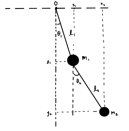
Before examining the code for the computer simulation, we will first solve for the equations of motion of the double pendulum using the Lagrangian method. Using the above figure, we see that we can write the Cartesian coordinates of the two masses in terms of the generalized coordinates, θ₁ and θ₂, so the position of the pendulum masses can be written as:

\begin{align} x_{1} = L_{1} \sin(\theta_{1}) \qquad y_{1} = - L_{1} \cos(\theta_{1}) \end{align}

\begin{align} x_{2} = L_{1} \sin(\theta_{1}) + L_{2} \sin(\theta_{2}) \qquad y_{2} = - L_{1} \cos(\theta_{1}) - L_{2} \cos(\theta_{2}) \end{align}

To obtain the velocities, we differentiate with respect with time to get:

\begin{align} \dot{x_{1}} = L_{1} \dot{\theta_{1}} \cos(\theta_{1}) \qquad \dot{y_{1}} = L_{1} \dot{\theta_{1}} \sin(\theta_{1}) \end{align}

\begin{align} \dot{x_{2}} = L_{1} \dot{\theta_{1}} \cos(\theta_{1}) + L_{2} \dot{\theta_{2}} \cos(\theta_{2}) \qquad \dot{y_{2}} = L_{1} \dot{\theta_{1}} \sin(\theta_{1})+ L_{2} \dot{\theta_{2}} \sin(\theta_{2}) \end{align}

The Lagrangian is given by subtracting the kinetic and potential energy (T and U, respectively): \(L = T - U\)

where T is given by: \begin{align} T&= \frac{1}{2} m_{1} v_{1}^2 + \frac{1}{2} m_{2} v_{2}^2 = \frac{1}{2} m_{1} (\dot{x_{1}^2} + \dot{y_{1}^2}) + \frac{1}{2} m_{2} (\dot{x_{2}^2} + \dot{y_{2}^2}) = \frac{1}{2} m_{1} L_{1}^2 \dot{x_{1}^2} + \frac{1}{2} m_{2} (L_{1}^2 \dot{\theta_{1} ^2} + L_{2}^2 \dot{\theta_{2}^2} + 2L_{1} \dot{\theta_{1}} L_{2} \dot{\theta_{2}} \cos(\theta_{1} - \theta_{2})) \end{align}

and U is given by: \begin{align}\begin{split} U &= m_{1} g y_{1} + m_{2} g y_{2}
&= -(m_{1} + m_{2}) g L_{1} \cos(\theta_{1}) - m_{2} g L_{2} \cos(\theta_{2}) \end{split}\end{align}

Subtracting T and U, we find that the Lagrangian of the system is: \begin{align} L = \frac{1}{2} (m_{1} + m_{2}) L_{1}^2 \dot{\theta_{1}^2} + \frac{1}{2} m_{2} L_{2}^2 \dot{\theta_{2}^2} + L_{2}^2 \dot{\theta_{2}^2} + m_{2} L_{1} \dot{\theta_{1}} L_{2} \dot{\theta_{2}} \cos(\theta_{1} - \theta{2}) + (m_{1} + m_{2}) g L_{1} \cos(\theta_{1}) + m_{2} g L_{2} \cos(\theta_{2}) \end{align}

Solving the Lagrange differential equation: \begin{align} \frac{\partial L}{\partial q} - \frac{d}{dt} (\frac{\partial L}{\partial \dot{q}}) = 0 \end{align}

For $\theta_{1}$, we get:

And for $\theta_{2}$, we get:

Since the time derivatives of $\theta_{1}$ and $\theta_{2}$ are the angular momentums $\omega_{1}$ and $\omega_{2}$, respectively, we can solve for $\ddot{\theta_{1}}$ and $\ddot{\theta_{2}}$ and rewrite them as:

\begin{align} \dot{\theta_{1}} = \omega_{1} \qquad \dot{\theta_{2}} = \omega_{2} \end{align}

\begin{align} \ddot{\theta_{1}} = \dot{\omega_{1}} = (m_{2}L_{1}\omega_{1}^2 \sin(\theta_{2}-\theta_{1}) \cos(\theta_{2}-\theta_{1}) + m_{2}g\sin(\theta_{2}\cos(\theta_{2} -\theta_{1}) + m_{2}L_{2}\omega_{2}^2\sin(\theta_{2}-\theta_{1}) - \frac{(m_{1} + m_{2}) g \sin(\theta_{1})}{(m_{1}+m_{2})L_{1} - m_{2}L_{1}\cos^2(\theta_{2} - \theta_{1})} \end{align}

\begin{align} \ddot{\theta_{2}} = \dot{\omega_{2}} = (-m_{2}L_{2}\omega_{2}^2 \sin(\theta_{2}-\theta_{1}) \cos(\theta_{2}-\theta_{1}) + (m_{1} + m_{2})g\sin(\theta_{1}\cos(\theta_{2} -\theta_{1}) - L_{1}\omega_{1}^2\sin(\theta_{2}-\theta_{1}) - \frac{g\sin(\theta_{2})}{(m_{1}+m_{2})L_{2} - m_{2}L_{2}\cos^2(\theta_{2} - \theta_{1})} \end{align}

Now having solved for these four differential expressions, we can begin writing the code.

import numpy as np
import matplotlib.pyplot as plt
import scipy.integrate as integrate
import matplotlib.animation as animation
from collections import deque

from numpy import sin, cos

We now define the initial conditions and constants for this problem as well as the parameters for the simulation, such as how much time should be simulated and how many trajectory points to display.

# define the constants
g = 9.8  # acceleration due to gravity in m/s^2
m1 = float(input("Enter mass 1 in kg: ")) # mass 1
m2 = float(input("Enter mass 2 in kg: "))  # mass 2
L1 = float(input("Enter length 1 in m: ")) # length 1
L2 = float(input("Enter length 2 in m: "))  # length 2
L = L1+L2
total_t = float(input("Enter total time in s: "))  # number of seconds to simulate
history_len = 50000  # number of trajectory points to display

# define initial values of theta1, theta2, angular momentum 1, and angular momentum 2
theta_1 = float(input("Enter theta 1 in degrees: "))
theta_2 = float(input("Enter theta 2 in degrees: "))
w1 = float(input("Enter angular velocity 1 in rad/s: "))
w2 = float(input("Enter angular velocity 2 in rad/s: "))

Next, we write a function (called derivs) that represents the four differential expressions we found earlier. Given the specified initial conditions, this function finds the time derivatives of $\theta_{1}, \theta_{2}, \omega_{1}, \omega_{2}$.

def derivs(system, t):
    """
    Finds the time derivatives of the thetas and angular momentums from the derived differential equations using 
    the Lagrangian. 
    
    Args:
        system: a 4-tuple of the initial values of (theta 1, angular momentum 1, theta 2, angular momentum 2)
        t: a time array
    
    Returns: a 4-tuple of the time derivatives of theta 1, angular momentum 1, theta 2, angular momentum 2
    """
    theta_1 = system[0]
    w1 = system[1]
    theta_2 = system[2]
    w2 = system[3]
    
    delta = theta_2 - theta_1
    
    dtheta_1 = w1
    dtheta_2 = w2
    domega_1 = (m2 * L1 * (w1**2) * sin(delta) * cos(delta) + m2*g*sin(theta_2)*cos(delta) 
                   + m2*L2*(w2**2)*sin(delta) - (m1+m2)*g*sin(theta_1))/((m1+m2)*L1 - m2*L1*(cos(delta))**2)
    domega_2 = (-m2*L2*(w2**2)*sin(delta)*cos(delta) + (m1+m2)*(g*sin(theta_1)*cos(delta)
                   - L1*(w1**2)*sin(delta)-g*sin(theta_2)))/ ((m1+m2)*L2 -m2*L2*(cos(delta))**2)
                   
    return(dtheta_1, domega_1, dtheta_2, domega_2)

This function will be used by the scipy.integrate.odeint function to solve for the theta and angular momentum values at specified time values given in the time array, t. The following section of code creates that time step array using the user’s specified total_t input. We then define the 4-tuple of theta 1, angular momentum 1, theta 2, and angular momentum 2 and convert it into radians. Then solve for the theta values for each time in the time array and store it under the variable gen_coords. To plot the simulation, we need to convert these general coordinates back into Cartesian coordinates, using equations 1 and 2 to do so.

# create an array of time steps 
dt = 0.02
t = np.arange(0, total_t, dt) 

# create a 4-tuple of theta 1, angular momentum 1, theta 2, and angular momentum 2 
# convert values in tuple to radians 
system = np.radians([theta_1, w1, theta_2, w2])

# use scipy.integrate.odeint function to solve for theta and angular momentum values for each timestep 
gen_coords = integrate.odeint(derivs, system, t)

# use the solved theta values to calculate the Cartesian coordinates 
# these values are used to plot the pendulum below
x1 = L1*sin(gen_coords[:, 0])
y1 = -L1*cos(gen_coords[:, 0])

x2 = L2*sin(gen_coords[:, 2]) + x1
y2 = -L2*cos(gen_coords[:, 2]) + y1

The following section of code creates the simulation of the double pendulum. It does not require a knowledge of the physics behind the system, but rather a good understanding of Matplotlib animations. We first create the figure that all of the plot elements will be plotted on, then create the plot elements so that at each time step, the animate function we have written will graph the position of the pendulum to trace out its trajectory.

%matplotlib notebook

fig = plt.figure(figsize=(5, 5))
ax = fig.add_subplot(autoscale_on=False, xlim=(-L - 1, L + 1), ylim=(-L-1, L+1))
ax.set_aspect('equal')
ax.grid()

line, = ax.plot([], [], 'o-', lw=2)
trace, = ax.plot([], [], '.-', lw=1, ms=2)
time_template = 'time = %.1fs'
time_text = ax.text(0.1, 0.9, '', transform=ax.transAxes)
history_x, history_y = deque(maxlen=history_len), deque(maxlen=history_len)


def animate(i):
    current_x = [0, x1[i], x2[i]]
    current_y = [0, y1[i], y2[i]]

    if i == 0:
        history_x.clear()
        history_y.clear()

    history_x.appendleft(current_x[2])
    history_y.appendleft(current_y[2])

    line.set_data(current_x, current_y)
    trace.set_data(history_x, history_y)
    time_text.set_text(time_template % (i*dt))
    return line, trace, time_text

 
ani = animation.FuncAnimation(
    fig, animate, len(gen_coords), interval=dt*1000, blit=True)
plt.show()

To download the interactive notebook, go here.

Results

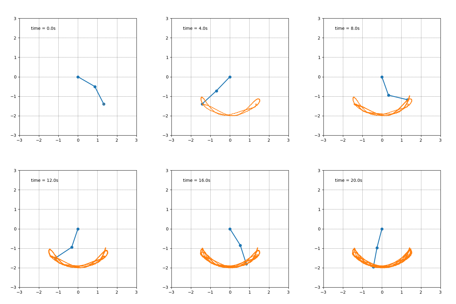
Here is an example of the resulting animation:

Discussion

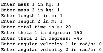
Putting the simulation to use, we input the following initial conditions:

After running the simulation with these initial conditions, we get:

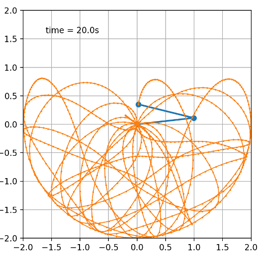
Clearly, just from looking at the completed path (the orange curves) of the pendulum, we can visually see that the its motion is chaotic and unpredictable, even though we know this is a deterministic system (after all, we were able to derive the four differential equations that represent this motion using the Lagrangian). The chaos of the system becomes even more apparent when we slightly change the initial conditions of the system. Now we have:

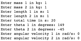
Where $\theta_{1}$ is now 149 degrees instead of 150 degrees.

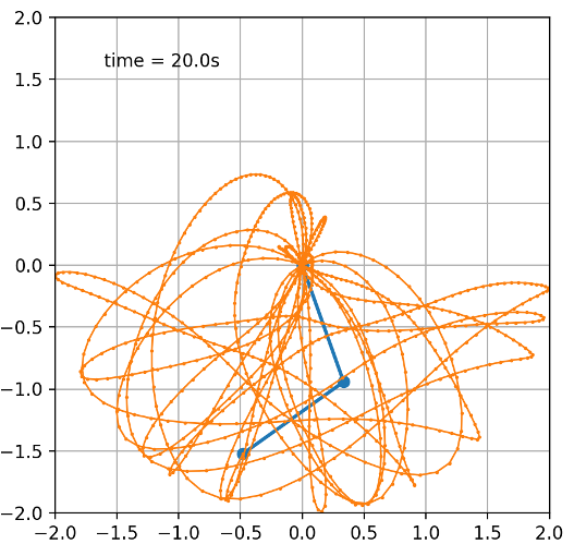
The picture above shows the trajectory of the double pendulum at the same time as the first simulation. Clearly, the motion of this pendulum is very different from that of the first one, even though the change in initial conditions was only by one degree, showing how vastly different the outcomes of a system can be with small deviations in initial conditions. We can further illustrate this property of chaotic dynamics, how tiny perturbations in initial conditions deviate into drastically different outcomes. Now, with an even smaller change in initial conditions, where $\theta_{1}$ is 149.9 degrees instead of 150 degrees:

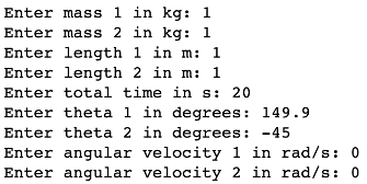
We get:

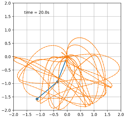
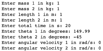
Once again, we can see that the motion of this pendulum is obviously different from that of the other two pendulums, despite that the initial conditions are only different from that of the first simulation by 0.1 degrees. We can reduce this order of this deviation in initial conditions further, where now, $\theta_{1}$ is 149.99 degrees instead of 150 degrees:

Which results in:

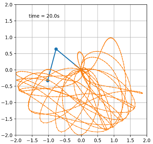
Although the beginning trajectory of the pendulum with these initial conditions was quite similar to that of the pendulum with $\theta_{1}$ of 150 degrees, around 10 seconds into the simulation, its trajectory quickly diverged, ultimately resulting in a trajectory path completely unique to these initial conditions. Of course, the computer calculation for the values of the thetas and angular momentums in itself could also have an effect on the chaotic and unpredictable behavior the system. Round off errors from finite arithmetic that are introduced when the computer uses approximations to calculate these theta and angular momentum values introduce tiny deviations in “initial conditions,” leading to potentially dramatically different outcomes in computer simulations of a chaotic deterministic system. This is another “source of chaos” that may lead to deviations in the pendulums’ trajectories hat may not be present in an infinitely precise simulation of a frictionless, double pendulum. It would be interesting to explore the effect of rounding errors and the limitations of computer calculations on the precision of computer simulated deterministic chaotic systems.

Chaos theory has applications in virtually every discipline, from the development of population models in biology and ecology to financial models in economics to weather prediction in meteorology to analyzing the motion of physical systems with classical mechanics.

Even with a comparatively simple system, the double pendulum, where we have further simplified things by assuming no friction and that the pendulum lengths are massless and rigid, we can and have clearly shown its inherent unpredictably and its extreme dependence on initial conditions. In other words, we have shown how even simple, deterministic systems can exhibit chaotic behavior.