Implementing Conway's Game of Life

The Game of Life, created by John Conway in 1970, is perhaps the best known example of cellular automaton. For those unfamiliar, cellular automaton is a collection of cells that live on a grid. Each cell has a state, and each cell has a neighborhood, which can be defined in any number of ways. At each time unit, each cell represents one of a finite set of states, and each update of a cell state is obtained by taking into account the states of the cells in its neighborhood. Cellular automaton are attractive because despite their apparent simplicity, they can be used to model various kinds of complex phenomena in many scientific fields, including biology, physics, and computer science.

Conway’s Game of Life is a zero-player game. In other words, the evolution of the grid of cells is determined by its initial state.

• The cells live on a grid that is a two-dimensional orthogonal grid of square cells. For the purpose of this implementation, this grid will be 100 by 100 squares.
• The cells have two possible states: live or dead.
• Every cell interacts with its eight neighbors (the cells that are horizontally, vertically, or diagonally adjacent).

The Rules

• Any live cell with fewer than two live neighbors dies (underpopulation).
• Any live cell with two or three live neighbors lives on to the next generation.
• Any live cell with more than three live neighbors dies (overpopulation).
• Any dead cell with exactly three live neighbors becomes a live cell (reproduction).

We can simplify these rules to have the following:

• Any cell with three neighbors survives.
• Any live cell with two neighbors survives.
• All other cells (dead or live) die in the next generation.

Implementing in Python

To begin, we will first load the necessary packages to create our implementation of the Game of Life. The NumPy library will be used to create our grid. Matplotlib’s Pyplot and Animation tools will be used to create the visualizations and animations of our game.

import numpy as np
import matplotlib.pyplot as plt
import matplotlib.animation as animation

Then, we will create the 100 by 100 grid that the cells live on by creating a NumPy array:

grid = np.random.binomial(1, 0.3, size=([100,100]))

Next, we create the function, called update, that will apply the rules to our cells and give us our updated grid. This function will be used by FuncAnimation to create an animation of the evolution of our cells. The nested for-loops in the code iterates through each cell in our grid and looks at the states of the cell’s neighbors. It does this by finding the sum of the neighboring cells’ states, where live = 1 and dead = 0. It then uses if statements to apply Conway’s rules to determine what the updated state of the cell should be.

def update(data):

    # make a copy of the current version of the grid
    global grid
    newgrid = grid.copy()
    
    # for loop applies Conway's rules to update state of the cell
    for i in range(100):
        for j in range(100):
            leftmost = max(0, j-1)
            uppermost = max(0, i-1)
            cell_value = grid[i,j]
            neighbor_sum = np.sum(grid[uppermost: i+2, leftmost: j+2]) - cell_value
            if neighbor_sum == 3:
                newgrid[i,j] = 1
            if neighbor_sum > 3 or neighbor_sum < 2:
                newgrid[i,j] = 0
    
    # used to display our animation of the grid
    mat.set_data(newgrid)
    grid = newgrid
    return [mat]

Finally, we can write the segment of code to create an animation of our game using FuncAnimation.

fig, ax = plt.subplots()
mat = ax.matshow(grid)
ani = animation.FuncAnimation(fig, update, frames = 200, interval = 100)
plt.show()

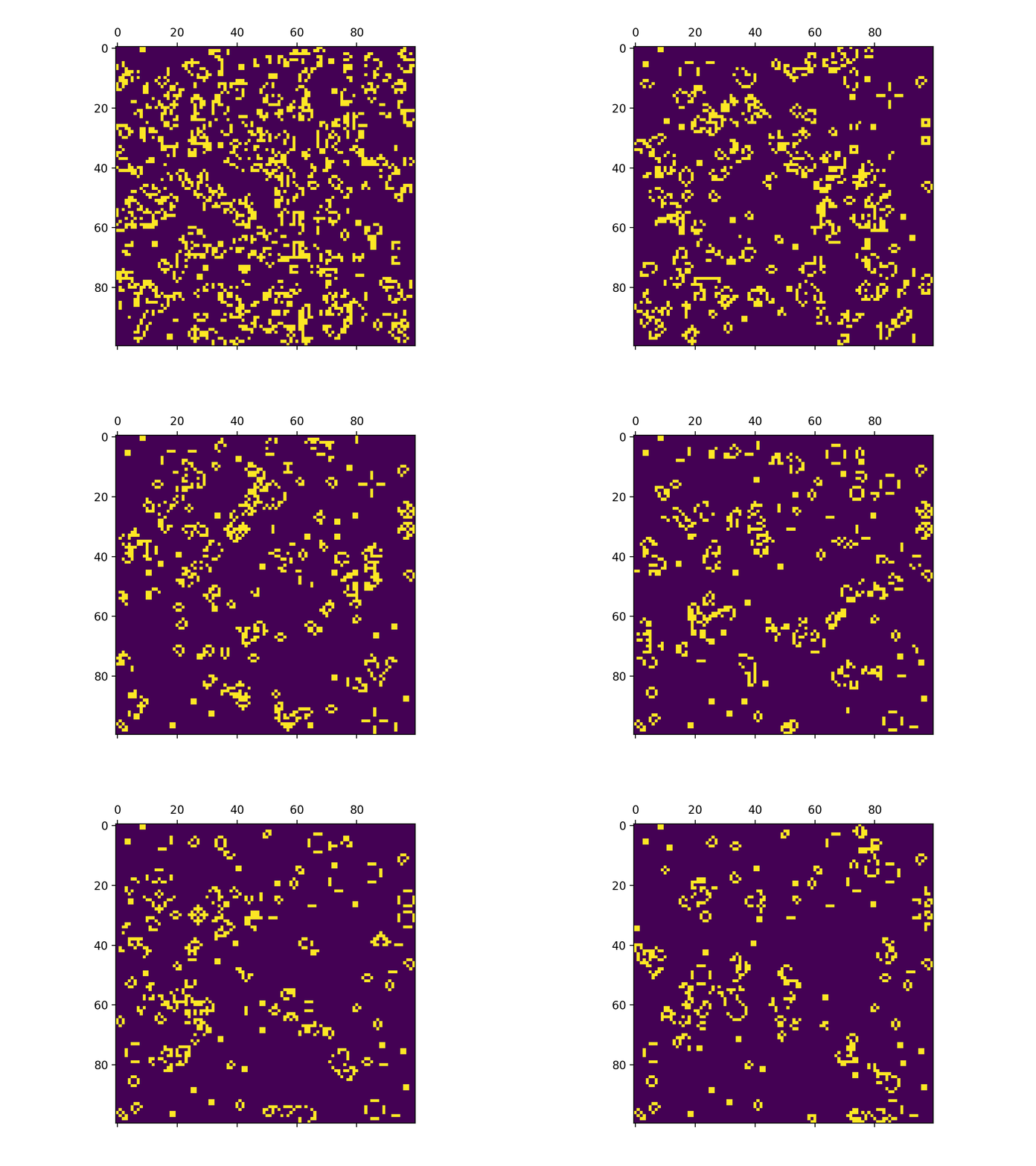
Below you will find a gif of the animation of one round of Conway’s Game of Life.