Visualization of tree cover and household income in Maricopa County, AZ

Having grown up in Arizona where summer temperatures regularly exceed 100 degrees Fahrenheit, I religiously follow two simple rules:

1. Avoid going outside between 10 AM and 4 PM.
2. If going outside is unavoidable, ALWAYS wear proper sun protection (sunscreen with minimum SPF 30, hats, sunglasses, the works) and seek shade.

Arizona has always been hot during the summer (no surprise there, it is located in the Sonoran desert after all), but climate change has made summer temperatures even more intense, not to mention worsening droughts and extending wildfire season for the rest of the Southwest. As a result, the risk of developing heat-related illnesses or death has also increased. Although the most effective way to avoid heat-related complications is by following rule 1, not going outside altogether during the day, what happens when you just can’t avoid going outside? That’s where rule 2 comes in. Whether you find shade from a man-made structure or naturally from tree cover, shade plays an important role in increasing your “thermal comfort” as temperature differences between shaded and unshaded surfaces may differ as much as 20-45 degrees F! And the air temperature in direct sunlight can feel 10-15 degrees warmer than it actually is in the shade.

Having established the importance of shade in staying healthy and comfortable in the heat, I wanted to explore the relationship between tree cover and social vulnerability (in this case, I looked at median household income) for zip codes in Maricopa County, Arizona.

Implementing in Python

To begin, we will first load the necessary packages to create our visualization of tree cover vs median household income. GeoPandas and Pandas will be used to use, manipulate, and visualize our geospatial data.

import geopandas as gpd
import pandas as pd

Then, we download the necessary data. From Google Earth Engine (https://earthengine.google.com/), I was able to download a GeoJSON file of the zip codes in Arizona and the mean tree cover per zip code. From the Census Bureau (https://data.census.gov/cedsci/), I downloaded a CSV table of household income information for Arizona zip codes. To only use the data for zip codes in Maricopa county, I also downloaded a text file of the zip codes and their corresponding county location from the Census Bureau. I stored the location of these files shown below:

path = "/Users/jessicazhang/Tree_vis/"

# file pathname for the GeoJSON file from Google Earth Engine
f_features = path + "az_features.geojson"

# file pathname for zip code and county information
fzip2county = path + "zip2county.txt"

# filepathname for income per zip code information
fincome = path + "Income2019/Income2019.csv"

Next, we use GeoPandas to read the features file:

az = gpd.read_file(f_features)
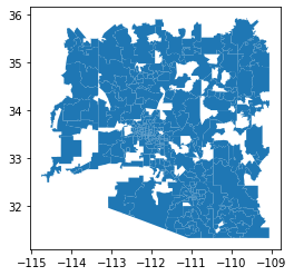
az.plot()

Note: we can see that the GeoJSON file includes the geospatial data for half of all zip codes in Arizona. Some zip codes are also missing. Since we’re only looking at Maricopa County, we need to use fzip2county to find the zip codes that are within Maricopa.

The fzip2county file looks like this:

221704257529619|01001|ZCTA5 01001|29247431|2127894|G6350|B5|S|27590249163642|25013|Hampden County|1598027523|44418900|G4020|H4|N|29247431|2127894
221704257529632|01002|ZCTA5 01002|137931897|4280973|G6350|B5|S|27590244937618|25011|Franklin County|1810941373|65609400|G4020|H4|N|9322298|215731
221704257529632|01002|ZCTA5 01002|137931897|4280973|G6350|B5|S|27590401060345|25015|Hampshire County|1365527344|46642098|G4020|H4|N|128609599|4065242
221704257529634|01003|ZCTA5 01003|2082670|14001|G6350|B5|S|27590401060345|25015|Hampshire County|1365527344|46642098|G4020|H4|N|2082670|14001

And contains zip code and county information for all US territories and states. To find only the zip codes in Maricopa County, we read fzip2county, iterating through each line in the file, adding the zip code to a list (maricopa_zips) if the zip code is within Maricopa County.

maricopa_zips = []
with open(fzip2county, 'r') as file:
    lines = file.readlines()
    for line in lines:
        if "Maricopa County" in line:
            maricopa_zips.append(line.strip().split('|')[2])    

So our list of Maricopa zip codes should look like this:

maricopa_zips = ['ZCTA5 85003', 'ZCTA5 85004', 'ZCTA5 85006', 'ZCTA5 85007', 'ZCTA5 85008', 'ZCTA5 85009', 'ZCTA5 85012', 'ZCTA5 85013', ...]

Since the fzip2county file (and income file later on) uses this notation for zip codes: ZCTA5 ##### and the GeoJSON file uses this notation: #####, to access the information in the GeoJSON file by zip code, we need to get rid of the ‘ZCTA5’ prefix in our maricopa_zips values:

maricopa_zip = []
for i in maricopa_zips:
    maricopa_zip.append(i[6:])

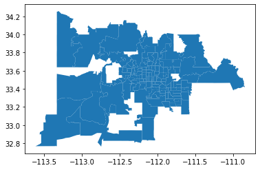
Let’s first verify that we’re on the right track. We do this by plotting the zip codes we’ve found. It should give us a plot of Maricopa County.

maricopa = az.loc[az['GEOID10'].isin(maricopa_zip)]
maricopa.plot()

This is indeed Maricopa County! Although because some zip codes were missing from the GeoJSON file, there are also missing zip codes in this plot of Maricopa County. For now, this isn’t a big issue as we have enough zip codes to work with.

Next, we read in the income information that we downloaded from the Census Bureau. Again, we only want data for zip codes in Maricopa County. And again, the income file uses this notation: ZCTA5 #####, so we need to use the list maricopa_zips, not maricopa_zip.

income = pd.read_csv(fincome)
income_maricopa = income.loc[income['NAME'].isin(maricopa_zips)

This income file contains a lot of information that isn’t useful for us. For this project, we only want to look at median household incomes. From the metadata, we find that this information is located in column ‘S1903_C03_001E’ of the fincome datatable.

income_maricopa = income_maricopa[['NAME', 'S1903_C03_001E']]
income_maricopa.rename(columns={"NAME": "ZCTA5CE10", "S1903_C03_001E": "Med_Income"}, inplace = True)

income_maricopa.drop(income_maricopa.index[income_maricopa['Med_Income'] == '-'], inplace = True)

for i, row in income_maricopa.iterrows():
    #print(row['ZCTA5CE10'])
    row['Med_Income'] = float(row['Med_Income'])
    row['ZCTA5CE10'] = row['ZCTA5CE10'][6:11]

In the code above, we’ve created a dataframe with two columns taken from the original fincome file, the zip code and median household income columns. This is the only pertinent information we need. I’ve also gone ahead and renamed the columns (from “NAME” to “ZCTA5CE10” and “S1903_C03_001E” to “Med_Income”) to better represent what each column represents. I’ve also converted the incomes in column “Med_Income” from strings to floats. Again, since the income file uses ZCTA5 ##### notation for zip codes, to make the GeoJSON dataframe (stored as maricopa) combatible to merge with our income dataframe (stored as income_maricopa), the last line of gets rid of the ‘ZCTA5’ prefix, allowing us to keep only the five digits in the zip code.

Now, let’s merge the maricopa and income_maricopa dataframes:

maricopa = maricopa.join(income_maricopa.set_index('ZCTA5CE10'), on = 'ZCTA5CE10')

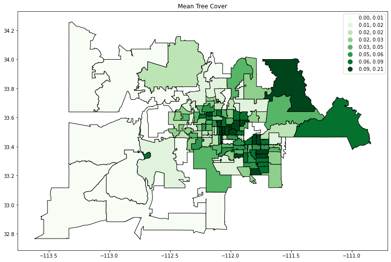
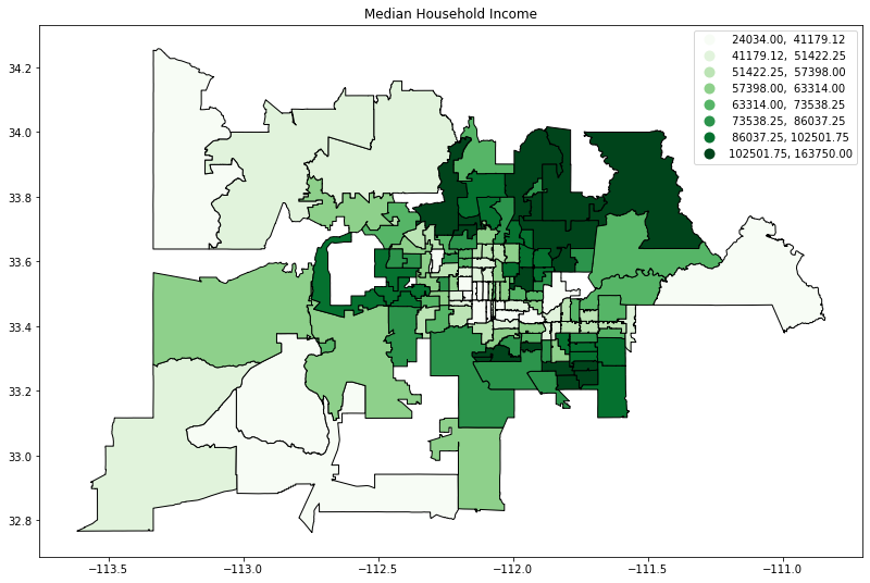
Finally, we can visualize this data!

ax1 = maricopa.dropna().plot(column = 'mean', cmap = 'Greens', scheme = 'Quantiles', k = 8,
                            figsize = (15, 9), 
                            legend = True, edgecolor = 'black').set_title('Mean Tree Cover')

ax2 = maricopa.plot(column = 'Med_Income', cmap = 'Greens', scheme = 'Quantiles', k = 8,
                            figsize = (15, 9),
                            legend = True, edgecolor = 'black').set_title('Median Household Income')